Econometric Modeling - Part 1

OLS

#

R-Square:

#

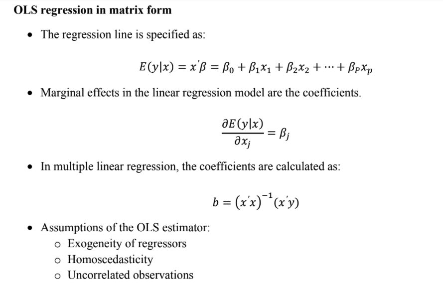
• The coefficient of determination (R-squared or R2) provides a measure of the goodness of fit for the estimated regression equation
• R2 = SSR/SST = 1 – SSE/SST
• Values of R2 close to 1 indicate perfect fit, values close to zero indicate poor fit.
• R2 that is greater than 0.25 is considered good in the economics field.
• R-squared interpretation: if R-squared=0.8 then 80% of the variation is explained by the regression and the rest is due to error. So, we have a good fit.

Adjusted $R^2$

#

R2 always increases when a new independent variable is added. This is because the SST is still the same but the SSE declines and SSR increases. Adjusted R-squared corrects for the number of independent variables and is preferred to R-squared.

where p is the number of independent variables, and n is the number of observations.

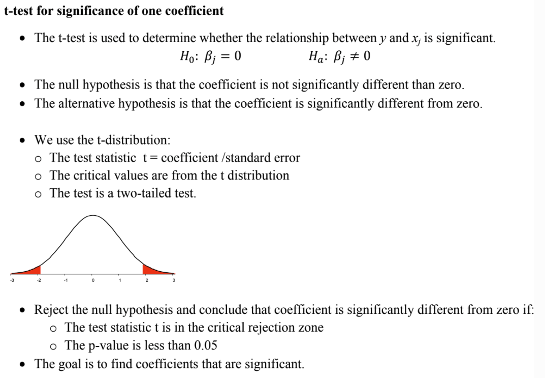
T-test for one coef:

#

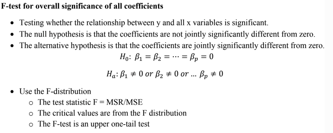
F-test for all coef:

#

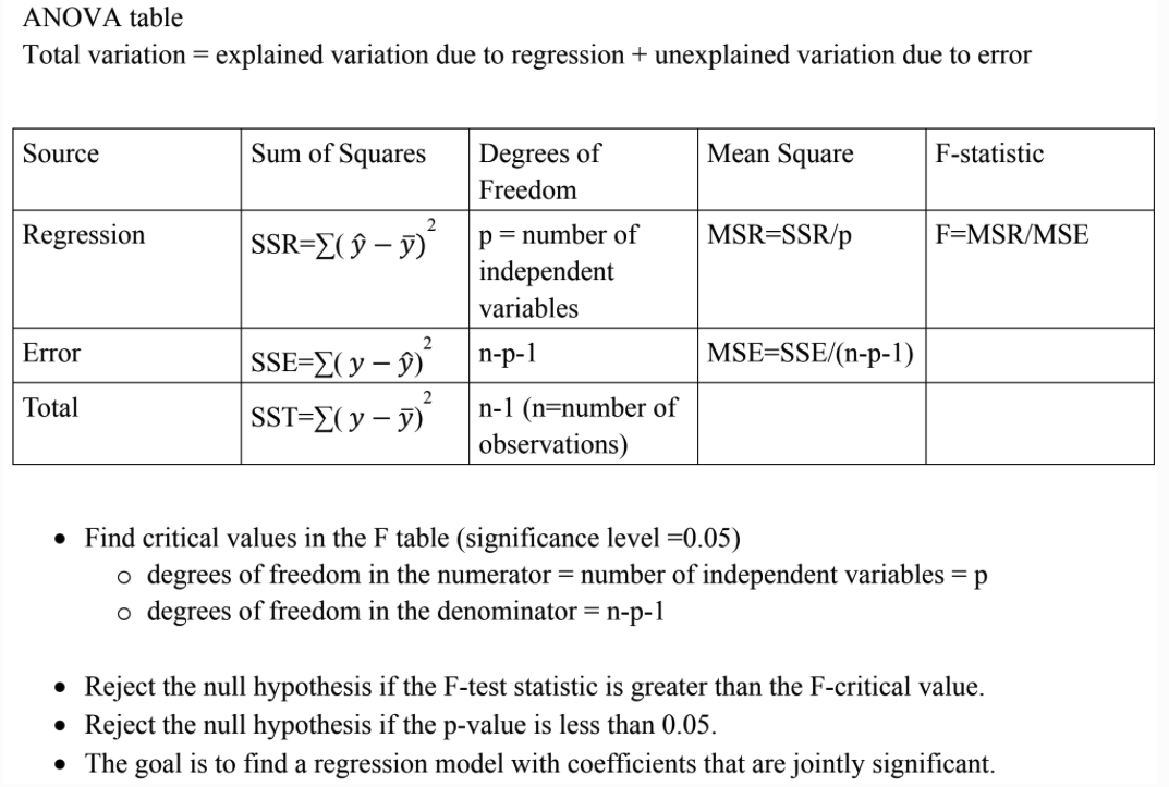
ANOVA Table

#

Linear Regression Assumptions:

#

Gauss Markov Assumptions are standard assumption for the LR model. If all assumptions satisfied, then OLS estimator is the best linear unbiased estimator of the coefficient,

• Linearity in parameter $\beta$ (however, x can be anything, i.e $x^2, log(x)$)

• Random Sampling. The data are a random sample drawn from the population

• No perfect collinearity(Can be detected by plotting correlation heat map, OR VIF, drop variable if $VIF_j >10$)

  • $$VIF_j = \frac{1}{1-R_j^2}$$

• Zero conditional mean(exogeneity) - regressors are not corrected with the error term. Endogeneity is a violation of the assumption where independent variable are correlated with the error term, can be handle with Instrumental Variables

  [!Note]

  The first four assumptions ensures that OLS estimater is unbiased, i.e.

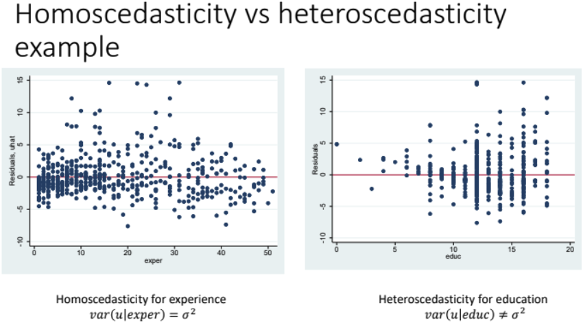
  $$ > E(\hat \beta_j) = \beta_j > $$

• Homoscedasticity: The variance of the error term u does not differ with the independent variable (we can check by plotting the residuals)

  • Consequence of Heteroscedasticity: The variance formula of OLS is no longer valid, t-test and F-test not valid, OLS is not BLUE.
  • To handle Heteroscedasticity, we can use Weighted Least Squares. If the Heteroscedasticity form is not known, the Feasible Generalized Least Square transforms the variable to get homoscedasticity.
  • LM-Test: $nR^2 \sim \chi_k^2$ , p>0.05 homo, otherwise hetero

• 

How to Compute OLS in R?

#

x <- c(1, 2, 3, 4, 5)
y <- c(2, 3, 5, 7, 11)

X <- cbind(1, x)  


XtX <- t(X) %*% X
XtY <- t(X) %*% y
beta_hat <- solve(XtX) %*% XtY
y_hat <- X %*% beta_hat


residuals <- y - y_hat
SSE <- sum(residuals^2)
SST <- sum((y - mean(y))^2)

# R²
R_squared <- 1 - SSE / SST

Time Series

#

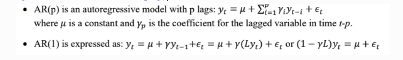
AR Model

#

Autoregressive (AR) models are models in which the value of a variable in one period is related to its values in previous periods.

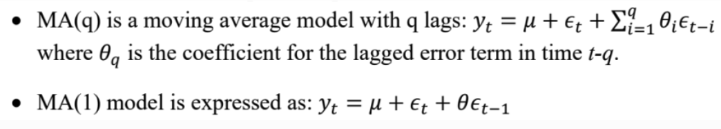
MA Model

#

Moving average (MA) models account for the possibility of a relationship between a variable and the residuals from previous periods.

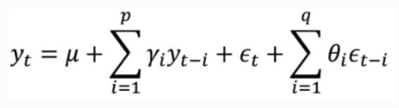
ARMA Model

#

Autoregressive moving average (ARMA) models combine both p autoregressive terms and q moving average terms, also called ARMA(p,q).

Stationarity

#

• Modeling ARMA(p, q) requires stationarity (an upward and downward trend means it is not stationary, need to differentiate at lag 1, e.g. $ARIMA(p, 1, q)$, making the first difference stationary process.
• Dick-Fuller Test for stationarity -> p>0.05 Non-Stationary

Seasonality

#

Seasonality is is a particular type of autocorrelation pattern where patterns occur every “season,” if there is a seasonal trend at lag 7, we should choose a $SARIMA(p, 1, q), (P, 1, Q)_7$ model

Box-Cox Transform

#

Use Box-Cox Transformation to stablize variance, this can handle the heteroskedasticity issue in our data, which improve the accuracy. The Box Cox use MLE to estimate the best lambda. If $\lambda = 1$ , no transformation needed. If $\lambda \rightarrow 0$, consider log transformation.

ACF and PACF

#

ACF is the proportion of the autocovariance of $y_t$ and $y_{t-k}$ to the variance of a dependent variable $y_t$. PACF is the correlation between $y_t$ and $y_{t-k}$ minus the part explain by the intervening lags.

• For an AR(p) model, the PACF is γ for the p lag and then cuts off.
• For an MA(q) model, the ACF is $\theta$ for the q lag and then cuts off.
• For an ARMA(p, q) model, both ACF and PACF changes gradually (no sudden decay to 0)
• For non-stationary model, ACF shows a slow decaying positive ACF, choose ARIMA(p, 1, q)
• For data with seasonarity, ACF show spike every s lag, choose $SARIMA(p, 1, q), (P, 1, Q)_s$

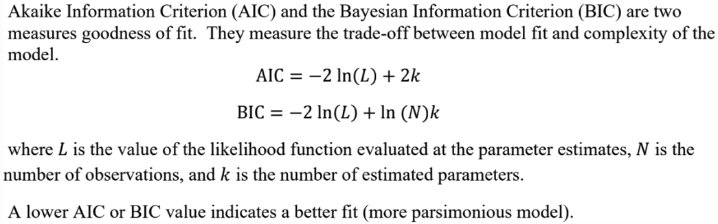
Model Selection with AIC and BIC

#

Diagnostic

#

• Check QQ plot for normality of the residual
• ACF and PACF show look like white noise
• Ljung Box Pierce test for magnitude of the autocorrelation of correlation as a group
• Check the roots of the AR and MA polynomials — either numerically or by plotting them on the unit circle. If they are both outside the unit circle, then it indicates stationarity(AR) and invertibility(MA)

Panel Data Models

#

Multiple time and mulitple variable:

• Varying regressors(annual income for a person, monthly food expenditures)
• Time-invariant regressors (gender, race, education)
• Individual-invariant regressor (time trend, US unemployment rate)

Variation: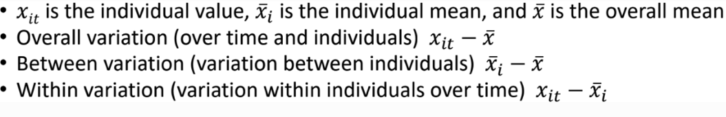

Pool OLS Estimator

#

Use when is homogeneous across individuals(rare in practice)

$N*T$ observations

Between Estimator

#

Uses cross sectional variation only: use when we interest in explaining the difference between two units (e.g. why one region uses more energy than another on average)

Drawback: Loses time series variation and cannot control for unobserved hetergeneity within units.

First Difference Estimator (FD)

#

Removes individual fixed effects by differencing data across time, use when the error term includes an individual-specific fixed effect, and serial correlation is not a concern.

Fixed Effects Estimator

#

Use when we believe unit-specific effects (e.g., regions, firms) are correlated with the regressors — for example, unobserved factors like income levels, regulation, or infrastructure that also affect energy usage, but it cannot estimate coefficients on time-invariant variables (e.g., population size if constant for each region).

Random Effects Estimator

#

Use when we believe those unit effects are uncorrelated with the regressors — which is a strong assumption. Assume: No correlation between unit effects and independent variables. Uses GLS (Generalized Least Squares); more efficient than FE if assumption holds.

Hausman Test

#

The Hausman test is used to decide whether to use the fixed effects (FE) or random effects (RE) estimator.