Scheduling 1 - Deterministric Model: Preliminaries

Table of Contents

Framework and Notation
#

For most of the scheduling problems, we consider finite number of jobs and finite number of machines. The number of jobs is denoted by n and the number of machines by $m$. Ususally, the subscript $j$ refer to a job while the subscript $i$ refers to a machine. If a jon requires a number of processing steps or operations, then the pair $(i,j)$ refer to the processing step or operation of job $j$ on machine $i$. A scheduling problem is typically defined using a triplet $\alpha | \beta| \gamma$

Processing Time $p_{ij}$: it represent the processing time of job j on machine i. The subscript i is omitted if the processing time of job j does not depend on the machine or if job j is only to process on one single machine.

Release date ($r_j$): The release date $r_j$ of job j may also be referred to as the ready date. It is the time the job arrives at the system, for example, the earliest time at which job $j$ can start its processing.

Due date($d_j$). The due date of job j represent the committed shipping or completion date (i.e. the date of the job is promised to the customer). Completion of a job after its due date is allowed, but then a penalty is incurred. When a due date must be met it is referred to as a deadline and denoted $\bar{d_j}$

Weight ($w_j$): The weight $w_j$ of job $j$ is basically a priority factor, denoting the importance of job j relative to the other job in the system.

Field	Description	Example
$\alpha$	Machine Environment (Single Entry)	$1$ (single machine), $P_m$ (Parallel Identical Machines), $J_m$ (Job Shop)
$\beta$	Processing Charateristics/Constraint (Zero or multiple entries)	$r_j$ (Release Dates), $prec$ (Precedence constraints), $s_{jk}$ (Sequence Depenedent Set up time)
$\gamma$	OBJ Function (Single Entry to be minimized)	$C_{max}$ (Makespan), $L_{max}$ (Maximum Lateness)

Possible Machine Environment $\alpha$
#

Single Machine (1)
#

The case of a single machine is the simplest of all possible machine environments and is a special case of all other more complicated machine environments.

Identical Machine in Parallel ($P_m$)
#

There are $m$ identical machines in parallel. Job $j$ requires a single operation and may be processed on any one of the $m$ machines or on any one that belongs to a given subset. If job $j$ cannot be processed on just any machine, but only on any one belonging to a specific subset $M_j$, then the entry $M_j$ appears in the $\beta$ field.

Machines in parallel with different speeds($Q_m$)
#

Threre are $m$ machines in parallel with different speeds. The speed of machine $i$ is denoted by $v_i$. The time $p_{ij}$ that job $j$ spends on machine $i$ is equal to $\frac{p_j}{v_i}$ (Assuming job $j$ received all its processing from machine $i$). This environment is referred to as uniform machines. If all machines have the same speed, i.e., $v_i = 1$ for all $i$ and $p_{ij}= p_{j}$, then the environment is identical to the previous one.

Unrelated machine in parallel($R_m$)
#

This environment is a further generalization of the previous one. There are $m$ different machines in parallel. Machine $i$ can process job $j$ at speed $v_{ij}$. The time $p_{ij}$ that job $j$ spends on machine $i$ is equal to $\frac{p_j}{v_i}$ (Assuming job $j$ received all its processing from machine $i$).. If the speed of the machines are independent of the jobs, i.e. $v_{ij} = v_{i}$, $\forall i, j$, then the environment is identical to the previous one($Q_m$)

Flow Shop ($F_m$)
#

There are $m$ machine in series. Each job has to me processed on each one of the m machines. All jobs have to follow the same route, i.e., they have to be processed first on machine 1, then on machine 2, and so on. After completion on one machine a job joins the queue at the next machine, Usually, all queues are assumed to operate under the First in Fist Out (FIFO) discipline: a job cannot “pass” another while waiting in a queue. If the FIFO discipline is in effect the flow shop is referred to as a permutation flow shop and the $\beta$ field should include prmu

Flexible flow shop ($FFc$)
#

A flexible flow shop is a generalization of the flow shop and the parallel machine environments. Instead of m machines in series there are c stages in series with at each stage a number of identical machines in parallel. Each job has to be processedfirst at stage 1, then at stage 2, and so on. A stage functions as a bank of parallel machines; at each stage job j requires processing on only one machine and any machine can do. The queues between the various stages may or may not operate according to the First Come First Served (FCFS) discipline. (Flexible flow shops have in the literature at times also been referred to as hybrid flow shops and as multi-processor flow shops.)

Job Shop (Jm)
#

In a job shop with m machines each job has its own predetermined route to follow. A distinction is made between job shops in which each job visits each machine at most once and job shops in which a job may visit each machine more than once. In the latter case the $\beta$-field contains the entry rcrc for recirculation.

Flexible job shop (FJc)
#

A flexible job shop is a generalization of the job shop and the parallel machine environments. Instead of m machines in series there are c work centers with at each work center a number of identical machines in parallel. Each job has its own route to follow through the shop; job j requires processing at each work center on only one machine and any machine can do. If a job on its route through the shop may visit a work center more than once,then the $\beta$-field contains the entry rcrc for recirculation

Open Shop (Om)
#

There are $m$ machines. Each job has to be processed again on each one of the $m$ machines. However, some of these processing times may be zero. There are no restrictions with regard to the routing of each job through the machine environment. The scheduler is allowed to determine a route for each job and diﬀerent jobs may have diﬀerent routes.

Possible Restriction and constraints $\beta$
#

Release dates ($r_j$)
#

If this symbol appears in the $\beta$ field, then job j cannot start its processing before its release date rj. If $r_j$ does not appear in the $\beta$ field, the processing of job j may start at any time. In contrast to release dates, due dates are not specified in this field. The type of objective function gives suﬃcient indication whether or not there are due dates.

Preemptions (`prmp`)
#

Preemptions imply that it is not necessary to keep a job on a machine, once started, until its completion. The scheduler is allowed to interrupt the processing of a job (preempt) at any point in time and put a diﬀerent job on the machine instead. The amount of processing a preempted job already has received is not lost. When a preempted job is afterwards put back on the machine (or on another machine in the case of parallel machines), it only needs the machine for its remaining processing time. When preemptions are allowed prmp is included in the $\beta$ field; when prmp is not included, preemptions are not allowed.

Predcedence Constraints (`prec`)
#

Precedence constraints may appear in a single machine or in a parallel machine environment, requiring that one or more jobs may have to be completed before another job is allowed to start its processing. There are several special forms of precedence constraints: if each job has at most one predecessor and at most one successor, the constraints are referred to as chains. If each job has at most one successor, the constraints are referred to as an intree. If each job has at most one predecessor the constraints are referred to as an outtree. If no prec appears in the $\beta$ field, the jobs are not subject to precedence constraints.

Sequence dependent setup times ($S_{jk}$)
#

The $s_{jk}$ represents the sequence dependent setup time that is incurred between the processing of jobs $j$ and $k$; $s_{0k}$ denotes the setup time for job k if job k is first in the sequence and $s_{j0}$ the clean up time after job $j$ if job $j$ is last in the sequence (of course, $s_{0k}$ and $s_{j0}$ may be zero) If the setup time between jobs $j$ and $k$ depends on the machine, then the subscript $i$ is included, i.e. $s_{ijk}$. If no $s_{jk}$ appears in the $\beta$ field, all setup times are assumed to be 0 or sequence independent, in which case they are simply included in the processing times.

Job families (`fmls`)
#

The $n$ jobs belong in the case to $F$ different job families. Jobs from the same family may have different processing times, but they can be processed on a machine one after another without requiring any setup in between. However, if the machine switches over from one family to another, say from family $g$ to family $h$, then a setup is required. If this setup time depends on both families $g$ and $h$ and is sequence dependent, then it is denoted by $s_{gh}$. If this setup time depends only on the family about to start, i.e. family h, then is denoted by $s_h$. If it doesn’t depend on either family, it is denoted by s.

Batch Processing (batch(b))
#

A machine may be able to process a number of jobs (b) simultaneously. It can process a batch of up to b jobs at the same time. The processing times of the jobs in a batch may not be all the same and the entire batch is finished only when the last job of the batch has been completed, implying that the completion time of the entire batch is determined by the job with the longest processing time. If $b = 1$, then the problem reduces to a conventional scheduling environment. Another special case that is of interest is $b = \infin$, i.e. there is no limit on the number of jobs the machine can handle at any time.

Breakdown (`brkdwn`)
#

Machine breakdowns imply that a machine may not be continuously available. The periods that a machine is not available are, in this part of the book, assumed to be fixed(e.g. due to shifts or scheduled maintenance).If there are a number of identical machines in parallel, the number of machines available at any point in time is a function of time, i.e., m(t). Machine breakdowns are at times also referred to as machine availability constraints.

Machine Eligibility Restrictions ($M_j$)
#

The $M_j$ symbol may appear in the $\beta$ field when the machine environment is $m$ machines in parallel ($P_m$). When the $M_j$ is present, not all $m$ machines are capable of processing job $j$. Set $M_j$ denotes the set of machines that can process job $j$. If the $\beta$ field does not contain $M_j$, job $j$ may be processed on any one of the $m$ machines.

Permutation(prmu)
#

A constraint that may appear in the flow shop enviroment is that the queues in front of each machine operate according to the FIFO discipline. This implies that the order (or permutation) in which the jobs go through the first machine is maintained throughout the system.

Blocking (block)
#

Blocking is a phenomenon that may occur in flow shops. If a flow shop has a limited buﬀer in between two successive machines, then it may happen that when the buﬀer is full the upstream machine is not allowed to release a completed job. Blocking implies that the completed job has to remain on the upstream machine preventing (i.e., blocking) that machine from working on the next job. The most common occurrence of blocking that is considered in this book is the case with zero buﬀers in between any two successive machines.

In this case a job that has completed its processing on a given machine cannot leave the machine if the preceding job has not yet completed its processing on the next machine; thus, the blocked job also prevents (or blocks) the next job from starting its processing on the given machine. In the models with blocking that are considered in subsequent chapters the assumption is made that the machines operate according to FIFO. That is, block implies prmu.

No-wait (`nwt`)
#

The no-wait requirement is another phenomenon that may occur in flow shops. Jobs are not allowed to wait between two successive machines. This implies that the starting time of a job at the first machine has to be delayed to ensure that the job can go through the flow shop without having to wait for any machine. An example of such an operation is a steel rolling mill in which a slab of steel is not allowed to wait as it would cool oﬀ during a wait. It is clear that under no-wait the machines also operate according to the FIFO discipline.

Recirculation (rcrc)
#

Recirculation may occur in a job shop or flexible job shop when a job may visit a machine or work center more than once.

Possible Objective Functions
#

Any other entry that may appear in the $\beta$ field is self explanatory. For example, $p_j = p$ implies that all processing times are equal and $d_j = d$ implies that all due dates are equal. Due dates, in contrast to release dates, are usually not explicitly specified in this field. The type of objective function give sufficient indication whether or not the jobs have due dates.

The objective to be minimized iss always a function of the completion times of the jobs, which depend on the schedule. The completion time of the operation of job $j$ on machine $i$ is denoted by $C_{ij}$. The time job $j$ exits the system (its completion time on that last machine on which it requires processing) is denoted by $C_j$. The objective may also be to a function of the due dates. The lateness of job $j$ is defined as

$$ L_j = C_j -d_j $$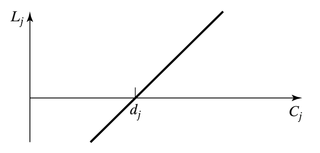

which is positive when job $j$ is completed late and negative when it is completed early. The tardiness of job $j$ is defined as

$$ T_j = \max(C_j - d_j, 0) = \max(L_j, 0) $$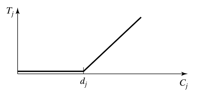

The difference between the tardiness and the lateness lies in the fact that the tardiness never is negative. The unit penalty of job j is defined as

$$ U_j = \begin{cases} 1 \text{ if } C_j > d_j \\ 0 \text { otherwise} \end{cases} $$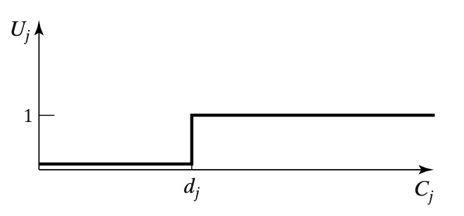

Makespan ($C_{max}$)
#

Makespan is defined as $\max(C_1, \dots, C_n)$, is equivalent to the completion time of the last job to leave the system. A minimum makespan usually implies a good utilization of the machines.

Maximum Lateness ($L_{max}$)
#

The maximum lateness, $L_{max}$, is defined as $max(L_1, \dots, L_n)$. It measures the worst violation of the due dates.

Total weighted completion time ($\sum w_j C_j$)
#

The sum of the weighted completion times of the n jobs give an indication of the totol holding or inventory cost incurred by the schedule. The sum of the completion time is also referred to as the flow time. The total weighted completion time is then referred to as the weighted flow time.

Discounted total weighted completion time ($\sum w_j (1 - e^{-rC_j})$)
#

This is a more general cost function than the previous one, where cost are discounted a rate of $r, 0 < r < 1$, per unit time. If job $j$ is not completed by time $t$ and additional cost $w_jre^{-rt}dt$ is incurred over the period $[t , t+dt]$. If job $j$ is completed at time t the total cost incurred over the period $[0,t]$ is $w_j (1- e^{-rt})$. The value of $r$ is usually close to 0, say 0.1 or 10%.

Total weighted tardiness ($\sum w_j T_j$)
#

This is also a more general cost function than the total weighted completion time.

Weighted number of tardy jobs ($\sum w_j U_j$)
#

The weighted number of tardy jobs is not only a measure of academic interest, it is often an objective in practice as it is a measure that can be recorded very easily.

All the objective functions above are so-called regular performance measures. A regular performance measure is a function that is nondecreasing in $C_1, \dots, C_n$. For example, when job $j$ has a due date $d_j$, it may be subject to an earliness penalty, where the earliness of job $j$ is defined as

$$ E_j = \max(d_j - C_j, 0) $$

This earliness penalty is non-increasing in $C_j$. An objective such as the total earliness plus the total tardiness, i.e.,

$$ \sum_{j=1}^n w_j'E_j + \sum_{j = 1}^n w_j''T_j $$

The weight associated with the earliness of job $j(w'_j)$ may be different from the weight associated with the tardiness of job $j(w''_j)$.

Example
#

A Flexible Flow Shop
#

$FFc|r_j|\sum w_jT_j$ denotes a flexible flow shop. The jobs have release dates and due dates and the objective is the minimization of the total weighted tardiness.

A Flexible Job Shop
#

$FJc|r_j,s_{ijk},rcrc|\sum w_jT_j$ refers to a flexible job shop with c work centers. The jobs have different release dates and are subject to sequence dependent setup times that are machine dependent. There is recirculation, so a job may visit a work centers more than once. The objective is to minimize the total weighted tardiness. Is is clear that this problem is a more general problem than the one described in the previous example.

A Parallel Machine Environment
#

$Pm |r_j, M_j|\sum w_jT_j$ denotes a system with $m$ machines in parallel. Job $j$ may be processed only on one of the machines belonging to the subset $M_j$. If job $j$ is not completed in time a penalty $w_jT_j$ is incurred.

A Single Machine Environment
#

$1|r_j, prmp|\sum w_jC_j$ denotes a single machine system with job $j$ entering the system at its release data $r_j$. Preemption are allowed. The objective to be minimized is the sum of the weighted completion times.

Sequence Dependent Setup Times
#

$1|s_{jk}|C_{max}$ denotes a single machine system with $n$ jobs subject to sequence dependent setup times, where the objective is to minimize the makespan. It is well-known that this problem is equivalent to the so-called Travelling Salesman Problem (TSP), where a salesman has to tour $n$ cities in such a way that the total distance traveled is minimized.

A Project
#

$P\infty| prec|C_{max}$ denotes a scheduling problem with $n$ jobs subject to precedence constraints and an unlimited number of machines (or resources) in parallel. The total time of the entire project has to be minimized. This type of problem is very common in project planning in the construction industry and has lead to techniques such as the Critical Path Method (CPM) and the Project Evaluation and Review Technique (PERT).

A Flow Shop
#

$Fm|p_{ij} = p_{j}|\sum w_jC_j$ denotes a proportionate flow shop environment with $m$ machines in series; the processing times of job $j$ on all $m$ machines are identical and equal to $p_j$ (Hence the term proportionate). The objective is to find the order in which the $n$ jobs go through the system so that the sum of the weighted completion times is minimized

A Job Shop
#

$Jm||C_{max}$ denotes a job shop problem with $m$ machine. There is no recirculation, so a job visits each machine at most once. The objective is to minimize the makespan. This problem is considered a classic in the scheduling literature and has received an enormous amount of attention.