Class of Distributions#
There are many statistical distributions that are useful in Six Sigma. They help us explain and analyze the shape of the data that will be encountered when designing and monitoring Six Sigma applications. They include:
- Normal
- Binomial
- Poisson
- T(students’s t)
- Chi Square
- F
We will skip this part for now as it will be revisited in other study notes in detail.
LCL, UCL, LSL, and USL#
When we consider quality, it is necessary to compare the inherent quality of the process with the expectation of the customer. The customer’s expectations can be measured by the lower specification limit (LSL) and upper specification limit (USL)
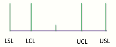
If the capabilities of the process (LCL and UCL) fall outside customer expectations (LSL and USL), the process has failed to deliver quality.
Here is an example of where the process variation is so large that customer expectations are occasionally not met. The distribution on top represents process variation. You can see that a small but still consequential percent of output falls below the LSL and above USL, such process does not reliably meet customer-based standards.
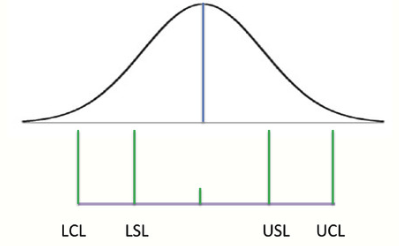
In a six sigma designed process, the mean of the distribution will be six standard deviations from the LSL and six standard deviation from the USL. This is the basis of six sigma designed process.
Near Perfect Outcomes#
We can therefore conclude that a Six Sigma designed process produces a negligible number of defects. It is so negligible that a process designed to this standard would be considered a near perfect process, one that delivers near perfect results.
Sigma and DPMO#
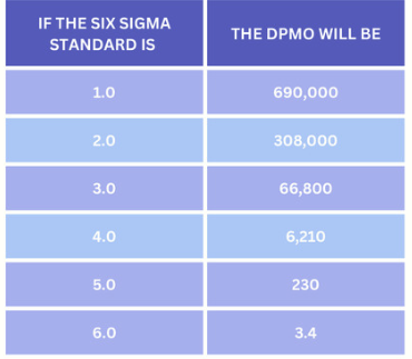
Below is the chart summarizing the number of Defect Per Million Opportunities for various levels of Sigma.
For a more common level of 4 sigma, there would be 6210 defects per million opportunities. This sounds like a substantial number of defects, but it is important to consider the output level for the process under consideration.
DPU#
Defect Per Unit (DPU) is the number of defects that have occurred in a sample divided by the number of units sampled.
$$ DPU = \frac{\text{Total number of defect in the sample}}{\text{Number of units sampled}} $$Using this measure of quality, a unit can have several defects. For example, in a sample of 50 orders(units) process by an online retailer, a single order had two wrong item sent to the customer. No other defect were found in the 49 remaining orders, So the DPU would be 2/50 or 0.04 defect per unit.
RTY and FTY#
RTY is Rolled Throughput Yield. It represents the likelihood that all of the steps in a process will be completed without any failure or rejects. For instance, if a process has 90 percent, the probability that all steps will be completed without failures is 90 percent.
FTY is First Time Yield, it is the number of good units, or pieces produced divied by the number of total units that originally started through the process. If 100 people started a training process, for example, but only 75 finished, then the FTY would be 75 percent.